Fast Prediction and Visualization
of Protein Binding Pockets with PASS
G. Patrick Brady, Jr.*
and Pieter F.W. Stouten1
*Experimental Station E500
Route 141 & Henry Clay Road
Wilmington, DE 19880-0500
G.Patrick.Brady@dupontpharma.com
Phone: (302)-695-3834
Fax: (302)-695-2209
1Present address:
Pharmacia & Upjohn
Viale Pasteur 10
20014 Nerviano (Mi)
Italy
Summary
PASS (Putative Active Sites with Spheres)
is a simple computational tool that uses geometry to characterize regions
of buried volume in proteins and to identify positions likely to represent
binding sites based upon the size, shape, and burial extent of these volumes.
PASS'S utility as a predictive tool for binding site identification is
tested by predicting known binding sites of proteins in the PDB using both
complexed macromolecules and their corresponding apo-protein structures.
The results indicate that PASS can serve as a front-end to fast docking.
The main utility of PASS lies in the fact that it can analyze a moderate-size
protein (~ 30 kD) in under twenty seconds, which makes it suitable for
interactive molecular modeling, protein database analysis, and aggressive
virtual screening efforts. As a modeling tool, PASS (i) rapidly identifies
favorable regions of the protein surface, (ii) simplifies visualization
of residues modulating binding in these regions, and (iii) provides a means
of directly visualizing buried volume, which is often inferred indirectly
from curvature in a surface representation. PASS produces output in the
form of standard PDB files, which are suitable for any modeling package,
and provides script files to simplify visualization in Cerius2®,
InsightII®, MOE®, Quanta®,
RasMol®, and Sybyl®. PASS is freely available
to all.
Keywords: protein active site,binding
site, cavity detection, buried volume, molecular modeling, computer-aided
drug design
Introduction
The identification and visualization of
protein cavities is the starting point for many structure-based drug design
(SBDD) applications. Sites of activity in proteins usually lie in cavities,
where the binding of a substrate typically serves as a mechanism for triggering
some event, such as a chemical modification or conformational change. Consequently,
binding sites are often targeted in attempts to interrupt molecular processes
via therapeutics. Although binding site locations are often furnished by
x-ray data or fold recognition, tools that automatically predict these
locations have become quite popular in SBDD, especially as front-ends to
molecular docking or when alternate binding sites are sought . The size
and shape of protein cavities dictates the three-dimensional geometry of
ligands that can strongly bind there; i.e. they must fit like a hand in
glove. Thus, a minimal requirement for drug activity is that the molecule
sterically fit the region of buried volume inscribing the active site cavity,
with some allowance for induced fit. The determination and visualization
of these volumes is critical in drug design, particularly since manual
intervention is still fruitfully employed in most design scenarios. An
ordinary stick representation of a protein, unfortunately, provides little
insight regarding the location, shape, or size of its buried volumes. While
surface representations are a step in the right direction, they still fall
short in that they require the user to infer buried volumes from often-occluded
void space. Consequently, methods for direct display of regions of buried
volume in proteins have become prevalent in recent years . Moreover, as
molecular docking and virtual screening become more predictive and prevalent,
the possibility of interfacing such tools with functional genomics via
threading or homology modeling becomes increasingly tempting. A versatile
tool that can rapidly predict binding sites should, therefore, find a niche
as a front-end to such automated screening efforts. This paper describes
a program called PASS (Putative Active Sites with Spheres), which may serve
both as an interface to virtual screening and as a visualization aid for
manual molecular modeling.
Methods
The PASS algorithm is designed to fill the cavities
in a protein structure with a set of spheres and to identify a few of these
spheres (called "active site points", ASPs) that most likely represent
the centers of binding pockets. Crevice filling is performed in layers
using three-point Connolly-like sphere geometry. An initial coating of
probe spheres is calculated with the protein as substrate, then additional
layers of probes are accreted onto the previously found probe spheres.
Only probes with low solvent exposure are retained, and the routine finishes
when an accretion layer produces no new buried probe spheres. Although
physical arguments can be made to substantiate PASS'S success in binding
site prediction, the algorithm itself is purely geometrical (see Figure
1).
Figure 1 - PASS Algorithm
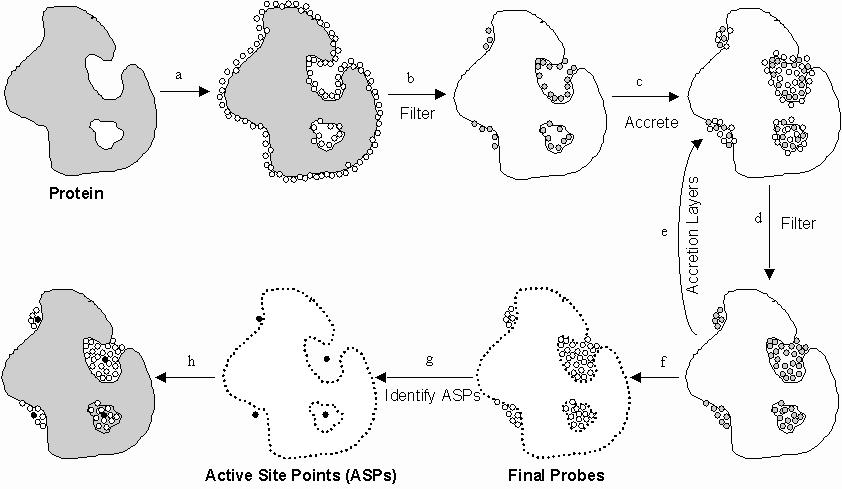
a. PASS uses three-point
geometry to coat the protein with an initial layer of spherical probes.
b. These probes are filtered to eliminate those that (i) clash with the
protein, (ii) are not sufficiently buried, and (iii) lie within 1Å
of a more buried probe. c. A new layer of spheres (white) is accreted onto
a scaffold consisting of all previously-identified probes (shaded). d.
The probes are filtered as described in step b. e. Accrete a new layer
of spheres onto the existing probes, as in step c. f. Accretion and filtering
(steps e and d) are repeated until a layer is encountered in which no newly-found
probes survive the filters. This leaves the final set of probe spheres.
g. Probe weights (PW) are computed for each sphere and active site points
(ASPs) are identified from amongst the final probes. h. The final PASS
visualization is produced. By default, the final probe spheres are first
smoothed, leaving only clusters of four or more.
Calculation of Probe Spheres
PASS begins by reading the Protein Data Bank
(PDB) coordinates of a target protein and assigning elemental atomic radii
(Table 1). Since a protein with explicitly represented hydrogen atoms contains
less interstitial volume than one without hydrogen, PASS assigns a few
different parameter values in the two cases. By default, if less that 20%
of the atoms in the protein PDB file are hydrogen, then all hydrogen atoms
are removed and hydrogen-free parameters are assigned; otherwise, hydrogen
is retained and hydrogen-inclusive parameters are assigned (Table 1). The
first layer of probe spheres is computed by looping over all unique triplets
of protein atoms and, if they are close enough together, calculating the
two locations at which a probe sphere (of radius Rprobe) may
lie tangential to all three protein atoms (Fig. 1; Step a). Appendix A
elucidates this three-point geometry, which is nontrivial since the radii
are not necessarily equal. To be retained, a putative probe sphere must
survive several filters (Fig. 1; Step b). The first condition is that it
cannot overlap with any atoms of the accretion substrate. The second filter
explicitly prohibits the probe from clashing with any protein atoms, while
the third ensures that the probe be somewhat buried within the protein
(i.e. in a binding-site-like region). In particular, each probe sphere
is ascribed a "burial count" (BC) representing the extent to which it is
excluded from solvent (Figure 2). The BC of a probe is computed by counting
the number of protein atoms that lie within a radius RBC=8Å
of it, and the probes are filtered such that any probe sphere with BC less
than a threshold value (BCthreshold) is rejected. This threshold
value was determined empirically, as were many of the PASS parameters,
by visual inspection of results for a few test systems. Our experience
has been that PASS'S predictions are largely insensitive to the precise
values of any of its parameters. Finally, probe spheres are "weeded" such
that no two probe centers lie any closer together than Rweed
= 1Å. This keeps the distribution of probe spheres from becoming
clumped, which enables reliable prediction of active site points from the
final set of probes.
Table 1 - PASS Parameters
| Parameter |
| Rprobe
hydrogen-free |
1.8 Å
|
| BCthreshold
hydrogen-free |
55
|
| Rprobe
with hydrogen |
1.5 Å
|
| BCthreshold
with hydrogen |
75
|
| RBC |
8.0 Å
|
| Rweed |
1.0 Å
|
| Raccretion |
0.7 Å
|
| Ro |
2.0 Å
|
| Do |
1.0 Å
|
| RASP |
8.0 Å
|
| PWmin |
1100
|
| Elemental
Radii |
| Hydrogen |
1.20 Å
|
| Oxygen |
1.52 Å
|
| Nitrogen |
1.55 Å
|
| Carbon |
1.70 Å
|
| Sulfur |
1.80 Å
|
Values of PASS parameters, which
are defined as follows. Rprobe - Radius of a probe sphere. BCthreshold
- Threshold burial count (BC) distinguishing a buried probe from an exposed
one. RBC - Radius used to compute burial counts. Rweed
- Minimal separation between probe spheres. Raccretion - Radius
of probes as they are accreted onto existing probes. Ro, Do
- Parameters defining the probe weight (PW) envelope function (see Fig.
2). RASP - Minimal distance between active site points (ASPs).
PWmin - Minimal PW for an ASP.
Figure 2 - Burial Counts
and Probe Weights
The burial count (BC) of
a probe sphere is obtained by counting the number of protein atoms that
lie within RBC=8Å of it. The probe weight (PW) of a sphere
is obtained by summing the BCs of neighboring probe spheres, scaled by
the distance-dependent envelope function shown above. Ro = 2.0
Å and Do = 1.0 Å.
After the seminal layer of probes is computed,
additional layers of spheres are iteratively accreted onto the existing
probe spheres. At each iteration, a set of new probe spheres is computed
as described above (Fig. 1; Steps c,e), but with a smaller probe radius
(Raccretion = 0.7Å) and with the set of all probe spheres
retained from previous layers as the accretion substrate. New probes, however,
must still maintain a center-to-center distance of at least Rprobe+ i
from
each protein atom, i (of radius i).
The aforementioned filters are imposed when the newly-found spheres are
combined with those retained from previous layers (Fig. 1; Step d). PASS
continues the accretion phase until a layer is encountered in which none
of the newly-found probe spheres survives the filters (Fig. 1; Step f).
The result of this procedure is that the cavities, invaginations, and internal
voids in the protein are filled with a set of fairly evenly-spaced probe
spheres, all of which are buried and none of which sterically clashes with
the protein. Furthermore, probes lying along the protein surface are packed
in ideal steric contact with three protein atoms.
i
from
each protein atom, i (of radius i).
The aforementioned filters are imposed when the newly-found spheres are
combined with those retained from previous layers (Fig. 1; Step d). PASS
continues the accretion phase until a layer is encountered in which none
of the newly-found probe spheres survives the filters (Fig. 1; Step f).
The result of this procedure is that the cavities, invaginations, and internal
voids in the protein are filled with a set of fairly evenly-spaced probe
spheres, all of which are buried and none of which sterically clashes with
the protein. Furthermore, probes lying along the protein surface are packed
in ideal steric contact with three protein atoms.
Active Site Point (ASP) Determination
PASS subsequently identifies a small number
of "active site points" (ASP) from amongst the final set of probe spheres
(Fig. 1; Step g). These ASPs are meant to represent potential binding sites
(i.e. centers of putative active sites) for ligands of arbitrary shape
and polar character. Thus, PASS conservatively views a protein binding
site as simply an invagination in the protein surface that is large enough
to accomodate a ligand and possesses substantial solvent-excluded volume
in which hydrophobic ligand moieties may be buried. ASPs are accordingly
selected by identifying the central probes in regions that contain many
spheres with high BCs. In particular, each probe is assigned a "probe weight"
(PW), which is proportional to the number of probe spheres in the vicinity
and the extent to which they are buried. The probe weight of the ith probe
is given by  , where the
envelope function, f(r), is shown in Figure 2. This is conceptually similar
to the solvation term of Stouten et al. , the premise of which is that
the solvation energy of an atom varies linearly with its exposure which,
in turn, is proportional to the unoccupied volume around it. The final
ASPs are determined by cycling through the probes in descending order of
PW, keeping only those with PW >= PWmin (=1100) that are separated
by a minimum distance RASP (= 8Å) from the ASPs already
identified. Finally, the set of ASPs is rank-ordered according to PW values.
These are PASS'S predicted binding sites.
, where the
envelope function, f(r), is shown in Figure 2. This is conceptually similar
to the solvation term of Stouten et al. , the premise of which is that
the solvation energy of an atom varies linearly with its exposure which,
in turn, is proportional to the unoccupied volume around it. The final
ASPs are determined by cycling through the probes in descending order of
PW, keeping only those with PW >= PWmin (=1100) that are separated
by a minimum distance RASP (= 8Å) from the ASPs already
identified. Finally, the set of ASPs is rank-ordered according to PW values.
These are PASS'S predicted binding sites.
PASS Output
The default PASS output consists of (i)
a PDB file containing the final set of probe spheres, (ii) a PDB file of
the ASPs, and (iii) a separate PDB file for each ligand that was optionally
read in (see below). By default, PASS "smoothes" the probe spheres before
writing the final set of "display" probes to a PDB file. In particular,
only probes with at least 4 display probes lying within 2.5Å are
written to file by default. Smoothing removes all but appreciable groupings
of probe spheres, leaving the final visualization less cluttered. Smoothing
can be suppressed via the command-line flag [-all]. PASS also produces
visualization scripts for several popular molecular modeling packages;
namely, Cerius2®, InsightII®, MOE®,
Quanta®, RasMol®, and Sybyl®.
These scripts, which are optionally produced via command-line flags (e.g.
[-InsightII]), simplify visualization by automatically loading, rendering,
and coloring the protein, probe spheres, ASPs, and ligands. PASS also displays
detailed runtime information, including parameter settings, an account
of sphere calculation and filtering (e.g. Table 2), and final probe sphere
and ASP data, including BCs and PWs. PASS can also read the coordinates
of bound ligands, either automatically from the protein PDB file (as HETATM
entries with different residue names), or as separate files via the command-line
flag [-ligand <filename.pdb>]. For each ligand, PASS computes the distance
from each ASP to the nearest ligand atom and to the ligand center of mass.
Other command-line options enable the user to (i) produce an enhanced set
of probe spheres and ASPs ([-more]), (ii) repress production of the probe
sphere PDB file ([-noprobes]), (iii) treat water molecules as part of the
protein ([-water]), rather than ignoring them (which is the default behavior),
(iv) specify an explicit output path ([-outdir <directory_path>]), (v)
produce a set of PDB files containing subsets of the final probe spheres
that were produced in the various layers of sphere calculation ([-layers]),
and (vi) compute the volumes of all groupings of probe spheres left after
smoothing ([-volume]). None of these options slows PASS noticeably except
the volume calculation, which proceeds as follows. After probe smoothing,
the final set of display probes is agglomeratively clustered by iteratively
merging pairs of overlapping groups of probes until an iteration attempts
to join two non-overlapping clusters. This determines both the optimal
number of probe groups and the identities of spheres in these groups. Group
volumes are subsequently computed by looping over probe spheres and estimating
the volume increments statistically. If ligand(s) are present, distances
are computed from the center of each group (i.e. the cluster center) to
(i) the nearest ligand atom (Dnear), and
(ii) the ligand center of mass (DCOM).
Table 2 - PASS Probe Sphere Algorithm
Applied to Thermolysin (1hyt)
| |
Layer #1
|
Layer #2
|
Layer #3
|
Layer #4
|
Layer #5
|
Layer #6
|
Layer #7
|
| Accretion
Substrate |
Protein
|
Probes
|
Probes
|
Probes
|
Probes
|
Probes
|
Probes
|
| Triplets
of Substrate Spheres Tried |
769,205
|
384
|
1,320
|
2,138
|
1,852
|
1,067
|
1,194
|
| Bridging
Spheres Found |
1,154,010
|
560
|
2,120
|
3,386
|
2,954
|
1,690
|
1,898
|
| ...
after substrate clash filter |
2,151
|
306
|
430
|
370
|
222
|
104
|
108
|
| ...
after protein clash filter |
2,151
|
118
|
115
|
88
|
53
|
16
|
14
|
| ...
after burial filter |
811
|
98
|
64
|
32
|
12
|
7
|
0
|
| ...
after weeding filter (New Probes) |
360
|
60
|
41
|
21
|
7
|
3
|
0
|
| Total
Probe Spheres |
360
|
420
|
461
|
482
|
489
|
492
|
492
|
| Comment |
Seminal Protein Coat
|
Accretion
|
Accretion
|
Accretion
|
Accretion
|
Accretion
|
Completion
|
The numbers of spheres retained
at various stages of a PASS calculation on thermolysin (1hyt). Protein
atoms form the substrate in the first layer; previously identified probe
spheres form the substrate in all subsequent layers. A triplet of substrate
spheres is tried if each substrate pair can be bridged by a probe sphere.
There are two possible probe sphere positions for each valid triplet of
substrate spheres. The number of bridging spheres found is always less
than twice the number of triplets tried because of exceptional cases (e.g.
one sphere lying inside the other two). The bridging spheres are then subjected
to a series of filters. The number of probes surviving the filters are
shown. Accretion procedes until a layer produces no new probes, which occurs
in the seventh layer in this case.
Results
Table 2 shows the numbers of probe spheres
retained at various stages of a PASS calculation on thermolysin (1hyt)
and is meant to provide an impression of the practical operation of the
algorithm. In layer #1 of the probe sphere calculation, the protein atoms
constitute the accretion substrate, and every set of three protein atoms
lying close enough together to be simultaneously touched by a single sphere
(of radius Rprobe) must be identified and used to determine
two putative probe sphere positions. The number of atomic triples that
must be tried is reduced by first identifying atomic neighborhoods. The
"neighborhood" of atom "i" is the set of atoms lying close enough to "i"
to be bridged by a single probe sphere. In layer #1, 769,205 triples of
protein atoms satisfied the neighborhood criterion, and 1,154,010 "bridging
spheres" were located using these triplets. The number of bridging spheres
is less than twice the number of atomic triples because not all triples
of atoms in the accretion substrate that satisfy the neighborhood criterion
can actually be bridged by a sphere of radius Rprobe. The set
of bridging spheres is then filtered according to (i) clash with the accretion
substrate, (ii) clash with the protein, (iii) burial count, and (iv) proximity
to other probe spheres, in that order. After the substrate clash filter,
2,151 putative probe spheres remain and, since the protein is the accretion
substrate in layer #1, the same number remains after the protein clash
filter. All but 811 putative probes are discarded based upon insufficient
burial, and 360 remain after these 811 are "weeded" to maintain a mutual
separation of at most Rweed=1.0 Å.
Thus, 360 probe spheres are found in the first layer. The accretion substrate
for the second and subsequent "accretion" layers is the set of probe spheres.
In layer #2, the substrate of 360 probe spheres requires that 384 substrate
triples be tested, from which 560 bridging spheres are identified. After
applying the four filters, only 60 new probe spheres remain, bringing the
total number of probes to 420 after layer #2. This process is repeated
until layer #7, in which no new probe spheres are identified, signalling
the completion of probe sphere determination. Note that although the number
of probe spheres continually grows as accretion procedes, the number of
accretion substrate triples that must be tried in each layer plateaus.
This is because PASS is written such that only triples of substrate atoms
incorporating a newly-found probe sphere (or the neighbor of a freshly-weeded
probe) are tried. As a result, PASS'S performance scales favorably with
protein size (approximately MW3/2
over
the molecular weight range in Table 3).
Table 3 - PASS Results for PDB Complexed
Proteinsa
|
PDB Code
|
Protein
|
Ligand(s)b
|
Size (kD)
|
Layers
|
Probes
|
ASPsc
|
Binding Site Hitsd
|
DNear
(Å)e
|
DCOM (Å)f
|
CPU Time (sec)g
|
|
1abe
|
l-arabinose binding
protein
|
l-arabinose
|
31
|
8
|
468
|
4
|
3
|
1.1
|
0.5
|
12
|
|
1bid
|
thymidylate synthase
|
DUMP
|
28
|
10
|
572
|
4
|
1
|
3.0
|
6.3
|
10
|
|
1cdo
|
alcohol dehydrogenaseh
|
NAD
|
37
|
8
|
760
|
7
|
2,3,5
|
1.4,3.2,0.9
|
4.2,11.3,9.8
|
13
|
|
1dwd
|
alpha thrombin + hirudin
|
NAPAP
|
31
|
7
|
664
|
7
|
1
|
0.6
|
4.7
|
11
|
|
1etr
|
epsilon thrombin
|
MQPA
|
32
|
6
|
774
|
16
|
2,15,16
|
0.8,1.3,2.4
|
5.1,5.5,6.6
|
11
|
|
1fbp
|
fructose-1,6 bisphosphataseh,i
|
F6P
AMP
|
32
|
6
|
593
|
5
|
3
-
(4)
|
1.8
-
(1.1)
|
3.9
-
(1.2)
|
12
|
|
1gca
|
galactose binding protein
|
d-galactose
|
32
|
5
|
575
|
9
|
1
|
0.7
|
0.8
|
11
|
|
1hew
|
lysozyme
|
NAG
|
13
|
8
|
211
|
1
|
1
|
0.7
|
6.9
|
5
|
|
1hvr
|
HIV 1 proteasei
|
XK263
|
20
|
10
|
385
|
2
|
1,2
|
1.2,0.8
|
2.3,6.3
|
8
|
|
1hyt
|
thermolysin
|
BZS
|
32
|
6
|
492
|
4
|
1
|
0.8
|
2.2
|
13
|
|
1inc
|
elastase
|
benzoxazinone
|
24
|
9
|
403
|
4
|
4
|
1.9
|
5.7
|
8
|
|
1jst
|
CDK2 - cyclin A complexh,j
|
ATP
|
59
|
7
|
1326
|
15
|
2
|
1.4
|
1.5
|
27
|
|
1pbe
|
p-hydroxybenzoate hydroxylase
|
FAD
PHB
|
41
|
10
|
935
|
10
|
1,2,6
-
(9)
|
1.5,1.0,0.8
-
(1.8)
|
7.2,12.6,2.5
-
(1.7)
|
16
|
|
1phf
|
cytochrome p450-camk
|
C4PI
|
43
|
7
|
723
|
6
|
1
|
0.7
|
0.9
|
17
|
|
1ppc
|
trypsin
|
NAPAP
|
22
|
5
|
304
|
2
|
1
|
1.0
|
4.8
|
6
|
|
1rbp
|
retinol binding protein
|
retinol
|
19
|
7
|
377
|
4
|
1,2
|
0.6,0.4
|
3.2,5.5
|
7
|
|
1rob
|
ribonuclease A
|
cytidylic acid
|
13
|
9
|
236
|
2
|
2
|
0.5
|
2.4
|
4
|
|
1stp
|
streptavidin
|
biotin
|
12
|
7
|
197
|
2
|
1
|
0.4
|
1.1
|
3
|
|
1ulb
|
purine nucleoside phosphorylasei
|
guanine
|
30
|
9
|
596
|
3
|
1
|
1.3
|
3.1
|
10
|
|
2er6
|
endothiapepsin
|
H256
|
31
|
7
|
487
|
3
|
1,2,3
|
1.9,1.0,0.8
|
8.7,7.6,1.2
|
11
|
|
2ifb
|
fatty acid binding protein
|
palmitic acid
|
14
|
6
|
292
|
3
|
1,2
|
0.4,0.8
|
1.8,6.6
|
5
|
|
2ptc
|
beta trypsin
|
PTI
|
22
|
5
|
305
|
2
|
1,2
|
1.1,2.6
|
19.4,19.8
|
7
|
|
2ypi
|
triose phosphate isomeraseh
|
PGA
|
25
|
9
|
486
|
5
|
4
|
3.4
|
5.7
|
8
|
|
3aah
|
methanol dehydrogenaseh,i
|
PQQ
|
64
|
7
|
997
|
8
|
4
|
0.5
|
3.1
|
30
|
|
3ptb
|
beta trypsin
|
benzamidine
|
22
|
6
|
290
|
2
|
1
|
0.9
|
0.8
|
7
|
|
4dfr
|
dihydrofolate reductaseh
|
methotrexate
|
17
|
8
|
366
|
3
|
1
|
3.9
|
8.1
|
5
|
|
4mbn
|
myoglobin
|
heme
|
16
|
5
|
297
|
3
|
1,2
|
0.8,0.5
|
5.4,5.9
|
5
|
|
4phv
|
HIV 1 protease
|
VAC
|
20
|
7
|
397
|
2
|
1,2
|
0.7,0.7
|
2.1,7.1
|
6
|
|
5cna
|
concanavalin Am
|
MMA
|
24
|
6
|
309
|
2
|
-
(3)
|
-
(0.3)
|
-
(1.4)
|
8
|
|
7cpa
|
carboxypeptidase A
|
FVF
|
32
|
6
|
481
|
3
|
2,3
|
0.6,1.0
|
6.5,3.1
|
14
|
aDefault
PASS parameters used; bound waters removed. Molecular weights do not include
hydrogen. Parenthetical entries were obtained in "more" mode (see text).
bLigand abbreviations:
DUMP = 2'-deoxyuridine 5'-monophosphate, NAD = nicotinamide adenine dinucleotide,
NAPAP = N==a==-(2-naphthyl-sulfonyl-glycyl)-DL-P-amidinophenylalanyl-piperidine,
MQPA = (2r,4r)-4-methyl-1-[Nalpha-(irs)-3-methyl-1,2,3,4-tetrahydro-8-quinolinesulfonyl)-L-arginyl]-2-piperidine
carboxylic acid,F6P = fructose 6-phosphate, AMP = adenosine monophosphate,
NAG = tri-n-acetylchitotriose, BZS = benzylsuccinic acid, ATP = adenosine-5'-triphosphate,
FAD = flavin-adenine dinucleotide, PHB = p-hydroxybenzoic acid, C4PI =
camphor 4-phenyl imidazole, cytidylic acid = cytidine 2'-monophosphate,
PTI = pancreatic trypsin inhibitor, PGA = 2-phosphoglycolic acid, PQQ =
pyrroloquinoline quinone, VAC = n,n-bis-2(r)-hydroxy-1(s)-indanyl-2,6-(r,r)-diphenylmethyl-4-hydroxy-1,7-heptandiamide,
MMA = alpha-methyl-d-mannopyranoside, FVF = bz-phe-val==p==(o)-phe. cNumber
of active site points (ASPs). dRank
of ASP(s) lying within 4 Å of the ligand. eDistances
from binding site hits to the nearest atom in the ligand. fDistances
from binding site hits to the center of mass of the ligand. gCPU
Times in seconds on a single Silicon Graphics R10000 processor running
at 194 MHz. hDimer
truncated to a monomer. iNo
water in the PDB file. jPhosphorylated
protein. kHeme treated
as part of the protein. mTetramer
truncated to a monomer.
PASS was first tested for its ability to
identify known binding sites. Table 3 shows the results of applying PASS
to 30 protein-ligand complexes drawn from the PDB. The structures were
chosen based upon diversity, resolution, inclusion in previous theoretical
studies, and the existence of corresponding apo-protein x-ray structures
in the PDB. In each case, hydrogen-free PASS parameters were assigned and
bound water molecules were ignored. For each PDB complex, Table 3 shows
the number of layers of probes PASS computed prior to convergence, the
final number of probe spheres, the number of ASPs identified for each protein
structure, and the required CPU time. Coordinates of the known ligand(s)
are used to define a binding site "hit." In particular, for each ASP of
a particular protein, two quantities are computed: (i) DNear,
the distance from the ASP to the nearest ligand atom, and (ii) DCOM,
the distance from the ASP to the ligand center of mass (COM). Any ASP with
DNear <= 4Å is considered a binding
site "hit." The Binding Site Hits column lists the rank order of the ASP(s)
that are considered hits, and the values in the DNear
and DCOM columns correspond to these
hits. For instance, the "1hvr" row in Table 3 indicates that both the top
ASP and the second-ranked ASP lie near the site in HIV-1 protease known
to bind XK263. In particular, the top ASP lies 1.2 Å from the nearest
XK263 atom and 2.3 Å from the COM, while the second-ranked ASP lies
0.8 Å from the nearest atom and 6.3 Å from the COM. Note that
ligand size impacts the DCOM values, as
evidenced by the trypsin-PTI system, which has the largest ligand (a protein)
and, correspondingly, the largest DCOM
values (~ 19 Å).
Table 3 shows that PASS is able to successfully
identify the locations of known binding sites in complexed x-ray structures.
PASS located the pocket containing a known ligand in all but three of the
32 trials, often finding multiple binding site hits for a given ligand
(11 times). In addition, the top-ranking ASP identified by PASS represents
a binding site hit in 19 of the 32 trials, and one of the top three ASPs
is a hit in 26 trials. These observations indicate that PASS can usually
identify the protein cavity to which a ligand will bind with maximal affinity
in a matter of seconds. There is a strong, but not perfect, correlation
between ASP rank (i.e. PW) and the volume of the corresponding group of
probe spheres. In fact, volume is approximately as predictive of binding
sites (results not shown) as ASP rank for the systems in Table 3. However,
the calculation of volumes slows PASS noticeably for systems requiring
many probe spheres (e.g. 92, 40, and 24 seconds for 1jst, 3aah, and 1etr,
respectively).
From a drug design perspective, the analysis
presented in Table 3 is somewhat immaterial, since the existence of complexed
coordinates implies that at least one binding site location is already
known. Intuition suggests that the presence of a ligand in a complex might
induce a more pronounced binding site cavity than would be present in an
apo-protein structure, thereby biasing a cavity-detection algorithm like
PASS to succeed on complexed systems. Thus, the postdiction of binding
sites in PDB complexes does not establish the predictive utility of a tool
for drug design, where one is lucky to have an apo x-ray structure or reliable
homology model.
A more realistic test of PASS as a tool
for prediction is to try to locate known binding sites on the structures
of proteins that are not complexed with a ligand. We address this predictability
issue by using PASS to compute ASPs for the set of apo-protein structures
from the PDB that correspond to complexed PDB structures in Table 3. Apo
structures were identified for as many of the systems in Table 3 as possible
(20), and default PASS parameters were used in all calculations. A few
of these PDB correspondences are not identical residue-by-residue because
the molecules either were obtained from different sources (1npc/1hyt; 2apr/2er6),
had residue additions or deletions at the termini (1swb/1stp; 1hxf/1dwd),
or had incomplete or missing residues due to poor electron density (5dfr/4dfr;
1hxf/1dwd). For comparison, the results displayed in Table 4 are presented
in the same order as in Table 3, and corresponding PDB codes are shown.
"Known" binding site positions are determined by superposing the native
and complexed structures and computing the proximity of the ASPs (from
the native PASS calculation) to the known ligand (from the complexed crystal
structure). This enables binding site "hits" to be computed as in Table
3, along with the distances DNear and DCOM
relating the position of the known ligand to the binding site hits. Only
backbone atoms {C,O,Ca,N} were superposed and, in all but a
few cases (see Table 4 caption), all residues in the chain were used. To
quantify how severely the ligand deforms the protein in the binding site,
we computed the RMSD between superposed structures using only residues
lying in this region. In particular, we identified both the set {Ci}
of residues lying within 4 Å of the ligand in the complex and the
set {Ai} of corresponding residues in the superposed apo structure.
The RMSD between {Ci} and {Ai} was then computed,
using both side chain and backbone atoms for identical amino acids and
only the backbone atoms otherwise.
Table 4 - PASS Results for PDB Apo-Proteinsa
|
Apo
PDB Code
|
Protein
|
Complex PDB Code
|
Probes
|
ASPsb
|
Binding Site RMSDc
|
Binding Site Hitsd
|
DNear
(Å)e
|
DCOM (Å)f
|
|
3tms
|
thymidylate synthase
|
1bid
|
577
|
4
|
1.7
|
1
|
3.9
|
6.8
|
|
8adh
|
alcohol dehydrogenase
|
1cdog
|
656
|
3
|
1.2
|
1,2
|
0.2,3.1
|
5.1,12.0
|
|
1hxf
|
alpha thrombin + hirudin
|
1dwd
|
627
|
8
|
0.7n
|
1,4
|
0.7,1.4
|
3.7,5.0
|
|
2fbpg
|
fructose-1,6 bisphosphatase
|
1fbpg
|
564
|
7
|
1.3
|
-
(9)
|
-
(1.9)
|
-
(4.8)
|
| |
|
|
|
|
|
-
(5)
|
-
(0.7)
|
-
(2.2)
|
|
1gcg
|
galactose binding protein
|
1gca
|
471
|
3
|
0.4
|
1
|
0.5
|
1.0
|
|
1hel
|
lysozyme
|
1hew
|
219
|
1
|
0.7
|
1
|
1.0
|
6.9
|
|
1npc
|
thermolysin
|
1hyt
|
455
|
3
|
1.7n
|
1
|
1.7
|
2.2
|
|
1esa
|
elastase
|
1inc
|
349
|
1
|
1.1
|
-
(4)
|
-
(0.3)
|
-
(4.6)
|
|
1brq
|
retinol binding protein
|
1rbp
|
401
|
2
|
2.2
|
1
|
0.9
|
3.4
|
|
8rat
|
ribonuclease A
|
1rob
|
216
|
2
|
0.6
|
1
|
0.3
|
1.8
|
|
1swbh
|
streptavidin
|
1stp
|
199
|
1
|
0.7n
|
1
|
0.8
|
2.4
|
|
1ula
|
purine nucleoside phosphorylase
|
1ulb
|
637
|
7
|
2.6
|
7
|
3.9
|
5.8
|
|
2apr
|
endothiapepsin
|
2er6
|
531
|
5
|
1.2n
|
2,5
|
1.5,0.9
|
2.6,9.0
|
|
1ifb
|
fatty acid binding protein
|
2ifb
|
291
|
4
|
0.6
|
1,2
|
2.5,0.9
|
4.6,4.1
|
|
3ptn
|
beta trypsin
|
3ptb
|
322
|
2
|
0.5
|
2
|
0.5
|
2.6
|
|
1ypig
|
triose phosphate isomerase
|
2ypig
|
508
|
7
|
2.4
|
3
|
2.2
|
2.0
|
|
5dfr
|
dihydrofolate reductase
|
4dfrg
|
283
|
2
|
1.3n
|
1
|
2.3
|
6.7
|
|
3phvj
|
HIV 1 proteasem
|
4phv
|
348
|
1
|
3.2
|
-
(1)
|
-
(1.0)
|
-
(5.1)
|
|
2ctv
|
concanavalin A
|
5cnah
|
361
|
4
|
1.1
|
2
|
0.6
|
1.0
|
|
5cpak
|
carboxypeptidase A
|
7cpak
|
448
|
3
|
2.0
|
1
|
1.2
|
4.6
|
aDefault
parameters used; bound waters removed. Parenthetical entries were obtained
in "more" mode (see text). bNumber
of active site points (ASPs). cAll
residues in the proteins were superposed (heavy backbone atoms only), except
where noted by superscript n. Binding site RMSDs are computed between all
residues that lie within 4 Å of the ligand in the complexed structure
and the corresponding residues in the apo structure (heavy atoms only).
Notation: 1abc (10,2) indicates that, for structure 1abc, the binding-site
RMSD calculation involved 12 residues, 10 of which included both backbone
and sidechain atoms, while 2 included only backbone atoms (since corresponding
residues were not of the same type). 3tms (12,0), 8adh (27,11), 1hxf (18,0),
2fbp (28,0), 1gcg (15,0), 1hel (11,0), 1npc (14,0), 1esa (14,0), 1brq (16,0),
8rat (8,0), 1swb (16,0), 1ula (8,0), 2apr (18,5), 1ifb (12,0), 3ptn (11,0),
1ypi (13,0), 5dfr (16,0), 3phv (26,0), 2ctv (9,0), 5cpa (18,0). dRank
of ASP(s) lying within 4 Å of the superposed ligand. eDistances
from binding site hits to the nearest atom in the superposed ligand. fDistances
from binding site hits to the center of mass of the superposed ligand.
gDimer
truncated to a monomer. hTetramer
truncated to a monomer. j3phv
dimer explicitly created via symmetry operators.
kZn
was considered part of the protein. mPASS
performed on dimer. nResidue
superpositions- 1hxf: {A44,F199,E217}; 1npc: {T2,G3,T4,F282,K308,V316}
of 1npc with {T2,G3,T4,F281,K307,V315} of 1hyt; 1swb: all residues except
{K134,P135} of 1swb (chain A) and {A13,E14,A15} of 1stp; 2apr: {S39,W42,I130}
of 2apr with {S36,W39,L128} of 2er6; 5dfr: {A6,N23,V93}.
Table 4 shows that PASS can reliably predict
binding site locations when only an apo x-ray structure is known. PASS
correctly identifies the binding site in 17 of the 21 trials in Table 4.
The top-ranked ASP hits the binding site in 12 trials, and one of the top
three ASPs is a hit in 16 trials. These observations imply that PASS may
be a suitable front-end to virtual high throughput screening and fast docking
routines. Furthermore, the similarity of observed hit rates between the
apo-protein and complexed systems refutes the hypothesis that the presence
of a ligand in the structural data is a crucial determinant of success
for a cavity detection algorithm.
One additional option available in PASS
is the generation of an enhanced set of probes
and ASPs by running PASS in "more" mode via the [-more] command-line flag.
In "more" mode, the burial count threshold is slightly reduced (by 10),
which typically has the effect of enhancing the number of probe spheres
by about a factor of two and ASPs by a factor of two or three, at the expense
of about 20-30% in cpu time. When the systems in Tables 3 and 4 are analyzed
in "more" mode, the binding site is detected in every case, with no ASP
hit ranking worse than ninth. Tables 3 and 4 show (in parentheses) the
ASP hits obtained in "more" mode for the few binding sites that the default
PASS calculation failed to locate. Detailed inspection revealed that several
of these default-mode misses contained an accumulation of probe spheres
that fell just beneath the threshold defining an ASP. Running PASS in "more"
mode is suggested when broad binding sites are anticipated (e.g. protein-protein
association).
The work of Mattos and Ringe constitutes
the experimental analog of PASS and enables the most direct comparison
of PASS to experimental data. In particular, Mattos and Ringe have soaked
elastase crystals with a variety of small organic solvents and crystallographically
determined the corresponding protein structures, including bound solvent
molecules. These bound organic probes are meant to map out potential binding
hot spots on the protein and suggest favorable ligand moieties. This raises
the question of whether their organic probes tend to cluster in regions
identified via PASS ASPs, which are likewise meant to identify possible
hot spots. To address this, PASS was run on elastase and the resulting
ASPs were graphically superimposed with Ringe et al.'s organic probes,
along with a set of bound ligands drawn from the PDB. Figure 3 shows these
results. Several clusters of organic probes are observed, most notably
a large grouping in the active site (S1 pocket). Although only one organic
probe lies within 8Å of the top- or second-ranked ASPs, PASS places
an ASP near four of the five largest clusters of probes. The inset to Figure
3 shows that the third-ranked ASP (pale blue) lies in the active site about
5Å above the catalytic triad (whose surface is colored green).
Figure 3 also addresses the question of
whether clusters of these experimentally derived organic probes are more
predictive of binding sites than PASS ASPs. Superposition of the ligands
from nineteen elastase PDB complexes enables this comparison. All but three
ligands bind in the S1 region of the known active site. The other three
stick solely to an alternate site about 10Å away (near S3'), while
four molecules employ both sites. PASS identifies this alternate binding
site via the fourth-ranked ASP (white); however, since only one organic
probe lies in this region, this site cannot be identified solely on the
basis of organic probe clusters. Conversely, there is a cluster of organic
probes near the S4 binding pocket, but no ASP is placed there (this region
is too close to the ASP in the S1 pocket). Thus, clusters of the organic
probes of Ringe et al. and the ASPs of PASS appear comparably predictive
of the known binding sites in elastase. It should be noted that the physical
nature of the probes employed by PASS and by Ringe et al. are drastically
different, so one should not expect identical distributions of binding
hot-spots in the two cases. Ringe et al. probe the protein surface with
small, often quite polar, molecules, precisely the opposite of PASS ASPs,
which can be thought of as large and apolar. ASPs are effectively apolar
in that they are identified solely on the basis of cavity size, shape and
burial, with no regard for e.g. electrostatics and hydrogen bonding. Moreover,
the PASS parameters have been tuned such that only a cavity of a certain
critical size can sustain an ASP. Over the set of systems in Table 3, the
smallest regions of buried volume containing an ASP are approximately the
size of a benzene ring, while ASP regions that bind a ligand are typically
three- to ten-fold larger than that. It is gratifying, however, that the
central binding site (S1) is unambiguously identified by both methods.
Figure 3 - Comparison
to Crystallographically-Determined Organic Probes
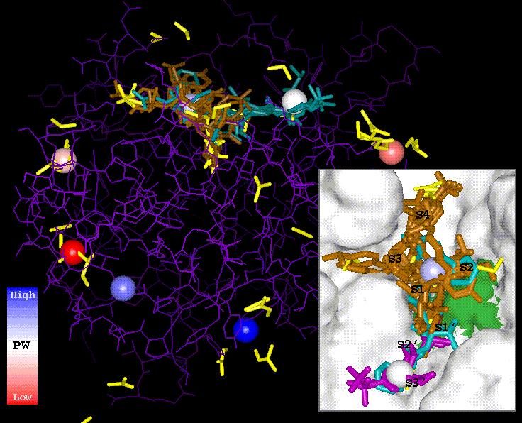
PASS was run in "more" mode
using a cross-linked structure of elastase provided by Ringe and Mattos.
The resulting ASPs are rendered as large spheres and colored according
to probe weight, PW (see scale). Crystallographically determined organic
probes (acetonitrile, dimethylformamide, acetone, ethanol, isopropanol,
hexenediol) are displayed as solid yellow sticks. Although only one organic
probe lies within 8Å of the top- or second-ranked ASP, four of the
five largest clusters of organic probes lie in a region identified as a
potential binding site by PASS. Every E.C.3.4.21.36 elastase complex in
the PDB (19 structures, 20 ligands: 1bma, 1btu, 1eai, 1eas, 1eat, 1eau,
1ela, 1elb, 1elc, 1eld, 1ele, 1elf, 1elg, 1esb, 1fle, 1inc, 1jim, 1nes,
9est) was superposed onto the cross-linked elastase structure, and the
resulting ligand overlays are shown as orange, blue, and magenta sticks
(except for two protein-bound structures, 1eai and 1fle). The inset shows
a top view of the protein surface at the active site, with the portion
of the surface defined by the catalytic triad colored green. The third-ranked
ASP (pale blue) is centrally located in the active site (S1 region), while
the fourth-ranked ASP (white) identifies an alternate binding site about
10Å away (S3' region). Only 4 ligands (two of which are proteins)
bind to both sites (colored blue). Thirteen of the twenty ligands (colored
orange) bind in the S1 pocket but not in the alternate site. The other
three ligands (1elf, 1elg, 1nes; colored magenta) bind only to the alternate
site. Since only one organic probe lies in this region, probe clusters
alone cannot identify this as a potential small molecule binding site.
Conversely, a cluster of three organic probes lies in the S4 region, in
a pocket that PASS failed to identify because it lies too close (i.e. <
RASP=8 Å) to
the S1 ASP.
Discussion
PASS in a Virtual Screening Environment
The hit rates shown in Table 4 indicate
that PASS may serve as a front-end to virtual screening when the binding
site is unknown or when alternative binding sites are sought. If the screening
tool is fast enough that docking against multiple sites is permissible,
then separate screening calculations can be run with the search space centered
on the top few PASS ASPs. This strategy should enable identification of
the optimal binding mode in most cases, as evidenced by the 71% hit rate
to the top two ASPs in Table 4. A number of other screening strategies
incorporating PASS are also possible. For instance, a more rigorous procedure
could be used to select the "true" binding site from amongst the full set
of ASP predictions. Using a docking routine with a more detailed scoring
function, the affinity of a ligand for the different ASP regions can be
directly compared. Thus, screening a small set of diverse probe molecules
or fragments against all the ASPs might enable one to identify the stickiest
region of the protein by comparing the scores of the top binders to each
ASP region. A large database of ligands could then be computationally screened
against this region. Since ASPs are determined using only steric size and
shape, the electrostatic (ES) and hydrogen-bonding (HB) character of the
ASP sites is arbitrary. One might, thus, search these sites for novel pharmacophores
and construct focused combinatorial libraries designed to hit them. Conversely,
one could use ES and HB characterization of ASP regions to select sites
most likely to possess affinity for a given class of compounds. Perhaps
the most alluring aspect of PASS'S speed is that it (i) permits the expeditious
analysis of entire structural databases (e.g. PDB, corporate), and (ii)
could provide a suitable bridge between 3D structural modeling and ligand
docking in a future drug design project designed to make use of genomic
data.
PASS as an Interactive Visualization
Tool
A PASS calculation on a moderate-sized
protein (~ 30 kD) takes less than twenty seconds on a single Silicon Graphics
R10000 processor (Table 3). PASS is, therefore, fast enough to be used
interactively in a molecular modeling environment, and has particular utility
as a visualization tool for drug design. By default, PASS produces PDB
files of probes, ASPs, and ligand(s) (when specified), which can be loaded
and rendered separately using any molecular modeling package. Alternately,
a full display of the PASS output can be produced in a single step (in
supported modeling suites) by executing a PASS visualization script, which
loads, renders, and colors the protein, probe spheres, ASPs, and ligand(s).
ASP coloring denotes probe weight (PW), while the probe spheres can be
colored according to either (i) burial count (BC), (ii) group identity
(optionally invoked via [-group]), or (iii) the layer of accretion in which
each was identified. Color values (0-50) are encoded onto the B-factor
column of the output PDB files containing the probes and ASPs. In runs
for which the probes are smoothed and grouped, an integer specifying the
group membership of each probe sphere is encoded onto the occupancy column
of the probe PDB file. Figure 4 shows a standard PASS visualization in
InsightII® for RNAse A (1rob), which is rendered as a tube
for clarity. The probes are rendered as small spheres and colored according
to BC, while the two ASPs are rendered as larger spheres and colored by
PW. The ligand, cytidylic acid, is shown in white and is mostly occluded
by probes and the second-ranked ASP. Because the ligand binds to a long
groove in the RNAse surface rather than a deep pocket, the ASP lying in
the true binding site has a lower PW than the one shown at the right, which
lies in a rounder cavity.
Figure 4 - PASS Visualization
of RNAse A

RNAse A (1rob) is shown
in green and is rendered as a tube for clarity, while the cytidylic acid
ligand is rendered in white sticks and is barely visible. The final probe
spheres, which have been smoothed, are represented by small spheres and
colored according to burial count. Active site points (ASPs) are rendered
as larger spheres and colored by probe weight. The second-ranked ASP lies
in the binding site.
One advantage of PASS as a visualization
tool is that displaying the ASPs relative to the protein enables immediate
identification of regions likely to be of interest in drug design. Since
the ASPs are centrally located in cavities, one can use the displayed ASPs
and a distance-based criterion to quickly identify the residues modulating
binding in these regions. For the modeling suites that support subseting
(e.g. InsightII), the PASS visualization scripts automatically define 6
Å, 8Å, and 10 Å residue-based subsets around each ASP,
which facilitate the coloring and specific display of these regions. Figure
5 shows the 8 Å subset of protein residues around the top-ranked
ASP of trypsin (3ptb). The ASP is shown in magenta, while the probe spheres
are colored by burial count. The residues involved in benzamidinium binding
are captured in this subset; e.g. hydrogen-bond partners are indicated
by yellow lines. The probe coloring clearly indicates that the mouth of
the binding pocket lies to the right, where the probe spheres have lowest
burial counts. Because PASS ASPs are centrally located in cavities, 6-10
Å radial subseting almost always enables selective visualization
of all the residues defining a protein cavity.
Figure 5 - Residues Modulating
the Binding of Benzamidinium to Trypsin
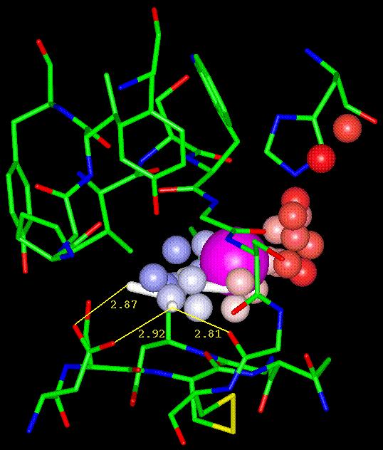
The residues lining the
binding pocket of trypsin (3ptb) are rendered as sticks and colored according
to atom type. They were selected by defining an 8 residue-based zone centered
on the top-ranked PASS active site point, shown in magenta. The bound benzamidinium
is shown in white, while the probe spheres near the pocket are rendered
as small spheres and colored according to burial count (BC). The BC color
scale runs from blue (high BC) to red (low BC), with muted colors denoting
intermediate values. Dashed lines represent hydrogen bonds between benzamidinium
and trypsin residues (D189 and G219), with distances measured in Angstroms.
By identifying multiple ASPs, PASS also
suggests alternate binding sites in proteins for which a primary site(s)
of binding has already been established. The pursuit of alternate binding
sites is becoming increasingly prevalent in light of the mounting realization
that many proteins have more than one biochemical role and are likely to
employ separate binding sites in performing distinct biochemical tasks.
In addition, many enzymes have allosteric binding sites that effect catalytic
activity or substrate binding via the induction of conformational changes
upon cofactor binding . PASS can suggest the locations of such sites. Finally,
the disruption of protein-protein interactions forms the basis of many
drug design efforts, and PASS can be used to identify interfacial pockets
that may be suitable targets for drug binding. In particular, interfaces
may be identified by using probe spheres to compute a difference map between
the bound and unbound forms. This approach can be extended to quickly identify
and visualize packing contacts in protein crystals or multimeric forms.
PASS also facilitates the visualization
of buried volumes in a protein in that the space occupied by the manifold
of probe spheres represents this volume, which can be viewed and manipulated
as a solid object by rendering the probes in a space-filling model. Mesh
or solid representations of various surfaces (molecular, van der Waals,
Connolly) are often used to visualize the shape complementarity of a protein
surface for putative ligands or functional groups. Often these surfaces
are colored according to some other receptor-based property, such as electrostatics,
hydrogen bond propensity, or surface curvature. The idea is that a modeler
can use this sort of display to look for likely ligand hot-spots on the
protein by visually searching the surface for voluminous invaginations
that are colored to indicate favorable complementarity in, say, electrostatic
potential. In reality, ligands only bind to regions possessing enough buried
volume to significantly accomodate them. Hence, buried volume is a quantity
of central importance in drug design, and the development of methods for
informatively displaying such regions should be accorded due attention.
Surface representations fail to capture buried volumes directly in that
the user is left to infer the buried volume from void space, much of which
is obscured from view by the surface. Likewise, colored surface quantities
are of most interest near deep invaginations, precisely where the surface
is most difficult to see. Unfortunately, user expertise is typically required
to overcome such difficulties. PASS takes a more direct approach by filling
the buried volumes with a set of unbonded atoms that represent the ASPs
and probe spheres. This enables both the size and shape of the buried volumes
to be viewed directly, either with or without the protein, using any molecular
visualization tool. Rendering the buried volumes as solid allows the user
to eyeball the fit of certain ligands and groups to potential hot-spot
regions. Figure 6 shows the region of buried volume (orange) lying in the
binding cavity of retinol binding protein (1rbp), along with the bound
retinol (white), some surrounding residues, and the top- and third-ranked
ASPs (in magenta), on the left and right, respectively. Information equivalent
to what is color-coded onto protein surface displays can, in principle,
be captured by property-based coloring of probe spheres. For instance,
the user could perform a finite-difference Poisson-Boltzmann calculation
and color the probe spheres according to electrostatic potential,
 es.
Directly displaying
es.
Directly displaying  es
in the region of interest, rather than having to infer it from
es
at the protein surface, provides a more meaningful view of electrostatics
than a surface representation. Favorable hydrogen-bond donor and acceptor
positions can likewise be more meaningfully defined within the manifold
of probe spheres than on a protein surface. Interaction-based coloring
schemes are not presently automated within PASS, however.
es
in the region of interest, rather than having to infer it from
es
at the protein surface, provides a more meaningful view of electrostatics
than a surface representation. Favorable hydrogen-bond donor and acceptor
positions can likewise be more meaningfully defined within the manifold
of probe spheres than on a protein surface. Interaction-based coloring
schemes are not presently automated within PASS, however.
Figure 6 - Buried Volume
in the Binding Pocket of Retinol Binding Protein

This view of the buried
volume inscribing the binding pocket of retinol binding protein (1rbp)
was obtained by rendering PASS probe spheres at 1.8 Å radius and
coloring them orange. The probes were rendered with slight transparency
in order to show the bound ligand (retinol) in white. The top- and third-ranked
ASPs, shown in magenta, appear on the left and right, respectively. Protein
residues lying within 8 Å of the two ASPs are diplayed in ball-and-stick
style and colored according to atom type.
Comparative Study
Many procedures for characterizing and
visualizing protein cavities have been presented in the past and, while
all differ substantially from PASS, comparative study serves to highlight
some of PASS'S strengths and weaknesses. First, almost all prior methods
identify cavity regions using some type of regular grid . A grid simply
provides the coordinates of points lying in cavities, which are then used
in some fashion to identify boundaries with the protein and, for all but
internal voids, with empty space. One disadvantage of using a grid is that
its storage consumes memory unnecessarily. Likewise, uncertainties arise
relating to the possible dependence of results upon grid spacing or positioning.
Orientational dependence was indeed found in the program POCKET . The advantage
of implementing a grid is purely algorithmic, as there is no physical reason
to use regular geometry when it is well known that protein packing and
protein surfaces are extremely irregular , if not fractal . The PASS algorithm
captures this irregularity by using geometry to project outward from the
known atomic coordinates in order to inscribe cavity regions. Although
this sort of protein-based approach has been taken by other groups , the
geometry employed in these studies differ significantly from PASS. Every
point in a protein cavity may be thought to represent a sphere that lies
exactly tangential to the protein surface. The radius of this sphere is
the distance of closest approach, and the sphere generally touches the
protein at one, two, or three points (i.e. atoms). Several authors have
used this correspondence (in reverse) to define points lying in cavity
regions by specifying a set of probe spheres and using geometry (one-,
two-, and/or three-point) to project outward from the protein atoms into
the cavity region. For instance, cavity points have been obtained by placing
tangential spheres midway between atoms and by rolling a probe sphere over
the set of atomic spheres representing the protein . The resulting probe
coordinates usually correspond to one or two points of tangency with the
protein. However, the sterically optimal packing of a spherical probe against
the protein has the probe lying tangent to exactly three atoms, just as
a marble that is dropped onto a pile of other marbles will come to rest
touching exactly three. Unlike any previous method, PASS uses only three-point
geometry to obtain points lying in cavity regions. Consequently, the shape
of the rendered manifold of PASS probes represents maximally favorable
sterics. One might expect that positioning the probe spheres using only
three-point geometry would give rise to a spotty distribution of probes
and poorly-shaped buried volume. Practical experience has shown, however,
that PASS produces smooth well-shaped buried volume manifolds (e.g. Figure
6), and that using only three-point geometry helps minimize the number
of points required to fill protein cavities.
The most ambiguous aspect of cavity characterization
lies in deciding where to place the boundary between the pocket and free
space; i.e. determining "sea-level" . Several studies appearing in the
literature operate by filling fully-enclosed volumes (e.g. "flood fill")
and, thus, require an artificial means of closing-off the mouths of cavities
in order to define sea-level. With many other methods , the definition
of sea-level arises as a biproduct of the algorithm itself and has no physical
significance. The work of Kuntz et al. is closest in spirit to the present
study with regard to sea-level definition. Their method uses the Connolly
surface as a substrate for sphere growth and rejects spheres based upon
two criteria: (1) an angular condition, which essentially selects concave
regions over flat or convex ones, and (2) a 5Å upper bound on radial
sphere growth. Their radial constraint is expected to generate sea-level
boundaries similar to those found with PASS. Unlike any other method of
cavity detection, however, PASS explicitly defines sea-level according
to a quantity of known physical significance, solvent accessibility, as
quantified by burial counts (BC).
Computational speed and ease of use are
also important criteria for comparison and, in these categories, PASS rates
favorably with all published methods. Although reliable speed comparison
is difficult since few studies report CPU times and others report times
on old processors , the fastest CPU times reported in the literature belong
to the LIGSITE program of Hendlich et al. , which can analyze a moderate-sized
protein (at 0.5 Å grid spacing) in about 15 seconds. This is approximately
the same speed demonstrated by PASS; however, the LIGSITE CPU time ramps-up
very steeply as the grid spacing is reduced (twelve-fold slower at 0.25
Å), and the authors provide only a cursory investigation of the dependence
of their results upon grid scale. PASS also excels in useability in that
it requires no startup cost to use because the inputs are simple and the
outputs are standard. A few programs in the literature appear to have shared
this design perspective . The input to PASS is restricted to a PDB file(s)
specifying the protein(s) coordinates plus a few optional command-line
flags that can be used to control more detailed behavior. PASS produces
versatile output in the form of standard PDB files, which allows the user
to immediately view the results using whatever modeling tool is already
familiar.
Physical Underpinnings
Although the roots of the PASS algorithm
are geometrical, not statistical mechanical, it is useful in light of PASS'S
success in identifying known binding sites to examine a posteriori which
physical interactions (if any) are mimicked in PASS. PASS takes the philosophy
that the task of binding site prediction is to identify regions of space
along the protein where an arbitrary ligand might tightly bind. A physically
well-designed algorithm should incorporate as many contributions to binding
affinity as possible without sacrificing applicability over a wide range
of ligands. Binding affinity is dictated by the free energy change induced
by the binding process,  Gbind,
which is known to have numerous contributions, both enthalpic and entropic.
While there is disagreement regarding some factors , sterics, electrostatics,
hydrogen-bonding, and solvation are known to be major players . Of course,
the fine details of ligand size, shape, flexibility, hydrogen-bonding propensity,
and polar character are crucial determinants of Gbind;
however, the observation that proteins usually bind ligands strongly at
only a few sites suggests that one might be able to use coarse details
of ligand character (e.g. size) to identify these few binding sites. Thus,
PASS must make its predictions using only binding affinity contributions
that depend upon coarse ligand character. Two important contributions to
Gbind
fit this description: solvation and sterics. Ligand binding
is always favored entropically by the desolvation of molecular moieties,
regardless of polarity . This is because the hydration of any atomic group
causes net ordering in the first few solvation shells of surrounding water.
The PASS algorithm mimics this desolvation effect via the rejection of
probe spheres based upon burial count. Likewise, the formation of steric
(i.e. enthalpic van der Waals) contacts between ligand and protein is generally
favorable, regardless of the ligand. Although the steric contribution to
Gbind
depends upon detailed molecular shape, the hardness of
the steric interaction precludes any ligand from binding tightly to the
protein without adopting a configuration consistent with the size and shape
of the buried volume. PASS includes sterics by imposing an implicit size
and shape criterion upon which regions of buried volume can be identified
as active site points (ASPs). In particular, a region of buried volume
that is either too small or too narrow to contain even a small ligand without
steric clash will never contain an ASP because too few probe spheres will
lie in the region for any one to have a large enough probe weight to be
selected as an ASP. The PASS parameters (esp. Ro and PWmin)
have been empirically tuned to make this distinction reliably.
Gbind,
which is known to have numerous contributions, both enthalpic and entropic.
While there is disagreement regarding some factors , sterics, electrostatics,
hydrogen-bonding, and solvation are known to be major players . Of course,
the fine details of ligand size, shape, flexibility, hydrogen-bonding propensity,
and polar character are crucial determinants of Gbind;
however, the observation that proteins usually bind ligands strongly at
only a few sites suggests that one might be able to use coarse details
of ligand character (e.g. size) to identify these few binding sites. Thus,
PASS must make its predictions using only binding affinity contributions
that depend upon coarse ligand character. Two important contributions to
Gbind
fit this description: solvation and sterics. Ligand binding
is always favored entropically by the desolvation of molecular moieties,
regardless of polarity . This is because the hydration of any atomic group
causes net ordering in the first few solvation shells of surrounding water.
The PASS algorithm mimics this desolvation effect via the rejection of
probe spheres based upon burial count. Likewise, the formation of steric
(i.e. enthalpic van der Waals) contacts between ligand and protein is generally
favorable, regardless of the ligand. Although the steric contribution to
Gbind
depends upon detailed molecular shape, the hardness of
the steric interaction precludes any ligand from binding tightly to the
protein without adopting a configuration consistent with the size and shape
of the buried volume. PASS includes sterics by imposing an implicit size
and shape criterion upon which regions of buried volume can be identified
as active site points (ASPs). In particular, a region of buried volume
that is either too small or too narrow to contain even a small ligand without
steric clash will never contain an ASP because too few probe spheres will
lie in the region for any one to have a large enough probe weight to be
selected as an ASP. The PASS parameters (esp. Ro and PWmin)
have been empirically tuned to make this distinction reliably.
Similar arguments cannot be made regarding
the electrostatic interaction, for instance, which may contribute either
attractively or repulsively to Gbind,
depending upon ligand
charge and polarity. Several other programs in the literature, however,
implement energetics in an effort to use other factors (e.g. hydrophobicity,
electrostatics) to help identify and rank potential binding site cavities
. Most notably, Ruppert et al. present the most impressive results in the
literature with regard to accuracy in locating binding sites . Their method
uses an in-house empirical forcefield to dock three different types of
probes (steric, H-bond donor, H-bond acceptor) against the protein binding
site. This maps out a set of favorable "probe" positions and permits the
identification of "sticky spots" on the protein, which are used as central
points to carve-out individual pockets. Although they provide no CPU times,
their algorithm requires significant docking and, thus, is probably considerably
slower than PASS or LIGSITE. They apply this method to the prediction of
binding sites in a set of 11 PDB complexes and find that their top-ranked
pocket contains the ligand in every case. Nine of these eleven cases, however,
are included in the PASS test set (Table 3), and strikingly similar results
are obtained with PASS. The top-ranked ASP is a binding site hit in eight
of the nine overlapping trials, and the second ASP is a hit in the other
case. Although factors such as electrostatics and hydrogen-bonding certainly
contribute to the affinity of a ligand for a particular cavity, the perspective
taken in PASS is that only the most ligand-independent contributions to
binding (i.e. size, shape, and burial extent of cavities) should contribute
to binding site prediction. Energetic factors that strongly modulate specificity
should be addressed case-by-case, either manually by the user or via downstream
software (e.g. docking). Thus, the PASS ASP regions are completely inclusive
with regard to electrostatic and hydrogen-bonding character, with the intention
that each will be reinvestigated individually in light of a particular
application or desired complementarity. PASS'S success in predicting binding
sites without electrostatics and hydrogen-bonding constitutes a remarkable
restatement of the importance of solvation and sterics in binding.
Conclusions
PASS is a simple cavity detection tool
that has utility in both virtual screening and interactive molecular modeling
environments. PASS was shown to reliably predict the locations of known
binding sites using a set of 20 apo-protein x-ray structures from the PDB,
thereby establishing its utility as a front-end to fast docking and virtual
screening. Furthermore, for the price of a thirty-second investment, PASS
provides the user a meaningful view of the buried volumes in a protein,
suggests alternate binding sites, and simplifies detailed visualization
of potential binding hot-spots. PASS is freely
available in unix executable form (SGI Irix, SunOS, Linux) to all users
via the Protein Data Bank web site under "PDB-related Software" (http://www.pdb.bnl.gov/pdb-docs/software.html).
Acknowledgements
The authors thank Carla Mattos and Dagmar
Ringe for providing their elastase structure with bound organic probes
and Zelda Wasserman for critical review of the manuscript. GPB thanks the
DuPont Pharmaceuticals Company for postdoctoral support during this work.
Appendix A - Three-Point
Sphere Geometry
The sphere placement algorithm in PASS
hinges upon solution of the following geometry problem. Given three "base"
spheres (i, j, and k) of known positions (Ri, Rj,
Rk)
and radii (i, j,
and k), at what two
positions (Rp) can a "probe" sphere of radius sp be placed
so as to be exactly tangential to all three base spheres? We seek the general
solution, in which none of the radii are necessarily equal and the coordinates
of the base spheres are unconstrained. Figure A1 illustrates the situation:
sphere perimeters are outlined, base sphere centers are labelled "i", "j",
"k", the "base plane" (i-j-k) is shaded, the probe sphere is shaded and
labelled "p", and vectors are denoted with uppercase lettering while points
and distances are in lowercase. The global origin coordinates is labelled
"O", while a local frame is defined by unit vectors {x´,
y´,
z´}.
There are, in general, two solutions for Rp, one on either
side of the base plane. However, one must first impose several conditions
to ensure the existence of a solution. If any pair {i,j} of base spheres
are too far apart, the probe will be unable to bridge the gap, so one must
first ensure that  , and
likewise for pairs {i,k} and {j,k}. One must also make sure that no base
sphere lies entirely within the volume occupied by the other two. With
these conditions satisfied, the coordinates Rp of the
two valid probe sphere positions may be written
, and
likewise for pairs {i,k} and {j,k}. One must also make sure that no base
sphere lies entirely within the volume occupied by the other two. With
these conditions satisfied, the coordinates Rp of the
two valid probe sphere positions may be written
 ,
(A.1)
,
(A.1)
where h is the height of the probe above
the base plane, and z´ is a unit normal to this plane. To
be precise, the local coordinate frame {x´, y´,
z´}
is right-handed, with x´ lying along Rj-Ri
and z´ pointing out of the base plane in the direction of
x´
x (Rk-Ri). The right triangle i-b-p
gives the height
 .
(A.2)
.
(A.2)
The vector Rb from O
to the point of projection of the probe onto the base plane, b, can be
written vectorially as
 ,
(A.3)
,
(A.3)
which leaves Tij and
U
undetermined. In general, point b need not lie on the interior of triangle
i-j-k, as drawn, but the equations are the same in either case.
U
can be eliminated from Eqn. (A.3) by observing that
 ,
(A.4)
,
(A.4)
where V º Tik
- Tij, and U points in the direction of y´.
Solving Eqn. (A.4) for U yields
 . (A.5)
The remaining vectors {Tij,
Tik,
Tjk},
which run from O to points {tij, tik, tjk},
are found by considering the triangles formed by two base spheres and the
probe sphere. For instance, the triangle i-j-p comprises two right triangles,
i-tij-p and j-tij-p. Applying the Pythagorean theorem
to each enables determination of the distance from i to tij
via a quadratic equation, which yields the desired vector
 .
(A.6)
.
(A.6)
Swapping indices in Eqn. A.6 gives analogous
equations for Tik and Tjk. The normal
vector, n, to the plane of tangency (a-b-g) may also be of interest:
 ,
(A.7)
,
(A.7)
where  ,
,  ,
and n is not of unit magnitude.
,
and n is not of unit magnitude.
Figure A1 - Sphere Geometry
